##  Family: gamma
##   Links: mu = log
## Formula: true_time ~ 1 + s_rmi * s_time_in_game + (s_rmi * s_time_in_game | level) + (s_rmi * s_time_in_game | subject)
##    Data: performance_and_rmi (Number of observations: 835)
##   Draws: 4 chains, each with iter = 4000; warmup = 2000; thin = 1;
##          total post-warmup draws = 8000
##
## Multilevel Hyperparameters:
## ~level (Number of levels: 10)
##                                          Estimate Est.Error l-95% CI u-95% CI Rhat Bulk_ESS Tail_ESS
## sd(Intercept)                                0.23      0.06     0.14     0.38 1.00     2565     3489
## sd(s_rmi)                                    0.02      0.01     0.00     0.04 1.00     2669     1910
## sd(s_time_in_game)                           0.01      0.01     0.00     0.04 1.00     2533     3800
## sd(s_rmi:s_time_in_game)                     0.01      0.01     0.00     0.03 1.00     4149     4281
## cor(Intercept,s_rmi)                         0.46      0.34    -0.34     0.93 1.00     6676     5487
## cor(Intercept,s_time_in_game)               -0.14      0.38    -0.81     0.63 1.00     9942     5403
## cor(s_rmi,s_time_in_game)                   -0.29      0.41    -0.90     0.63 1.00     5304     5291
## cor(Intercept,s_rmi:s_time_in_game)          0.14      0.43    -0.71     0.86 1.00     9581     5886
## cor(s_rmi,s_rmi:s_time_in_game)              0.14      0.43    -0.73     0.86 1.00     8054     6433
## cor(s_time_in_game,s_rmi:s_time_in_game)    -0.12      0.44    -0.85     0.75 1.00     6382     6267
##
## ~subject (Number of levels: 87)
##                                          Estimate Est.Error l-95% CI u-95% CI Rhat Bulk_ESS Tail_ESS
## sd(Intercept)                                0.16      0.01     0.14     0.19 1.00     1438     2902
## sd(s_rmi)                                    0.03      0.01     0.02     0.05 1.00     1727     2814
## sd(s_time_in_game)                           0.03      0.01     0.01     0.05 1.01     1216      922
## sd(s_rmi:s_time_in_game)                     0.02      0.01     0.00     0.04 1.00     1640     2897
## cor(Intercept,s_rmi)                         0.30      0.18    -0.05     0.64 1.00     5960     5075
## cor(Intercept,s_time_in_game)                0.22      0.20    -0.18     0.60 1.00     7303     3805
## cor(s_rmi,s_time_in_game)                    0.35      0.28    -0.25     0.84 1.00     2225     2714
## cor(Intercept,s_rmi:s_time_in_game)          0.17      0.31    -0.51     0.75 1.00     7964     4376
## cor(s_rmi,s_rmi:s_time_in_game)              0.52      0.36    -0.42     0.95 1.00     2757     3914
## cor(s_time_in_game,s_rmi:s_time_in_game)     0.21      0.38    -0.59     0.84 1.00     4313     5722
##
## Regression Coefficients:
##                      Estimate Est.Error l-95% CI u-95% CI Rhat Bulk_ESS Tail_ESS
## Intercept                5.05      0.08     4.89     5.20 1.00     1526     2545
## s_rmi                   -0.02      0.01    -0.04    -0.00 1.00     4257     5536
## s_time_in_game          -0.00      0.01    -0.02     0.01 1.00     6664     5278
## s_rmi:s_time_in_game     0.00      0.01    -0.01     0.02 1.00     6316     5456
##
## Further Distributional Parameters:
##       Estimate Est.Error l-95% CI u-95% CI Rhat Bulk_ESS Tail_ESS
## shape    67.84      4.36    59.68    76.86 1.00     2583     4408
##
## Draws were sampled using sampling(NUTS). For each parameter, Bulk_ESS
## and Tail_ESS are effective sample size measures, and Rhat is the potential
## scale reduction factor on split chains (at convergence, Rhat = 1).Game
Here is a video playthrough of each level.
Check out how data are tracked in real time.
Model
Here is where you can view more detail of the final model I summarized on the poster.
Model was fit with the brms package in R version 4.5.1. Visualization were completed using the ggplot2, tidybayes, bayesplot, and marginaleffects packages.
Model summary
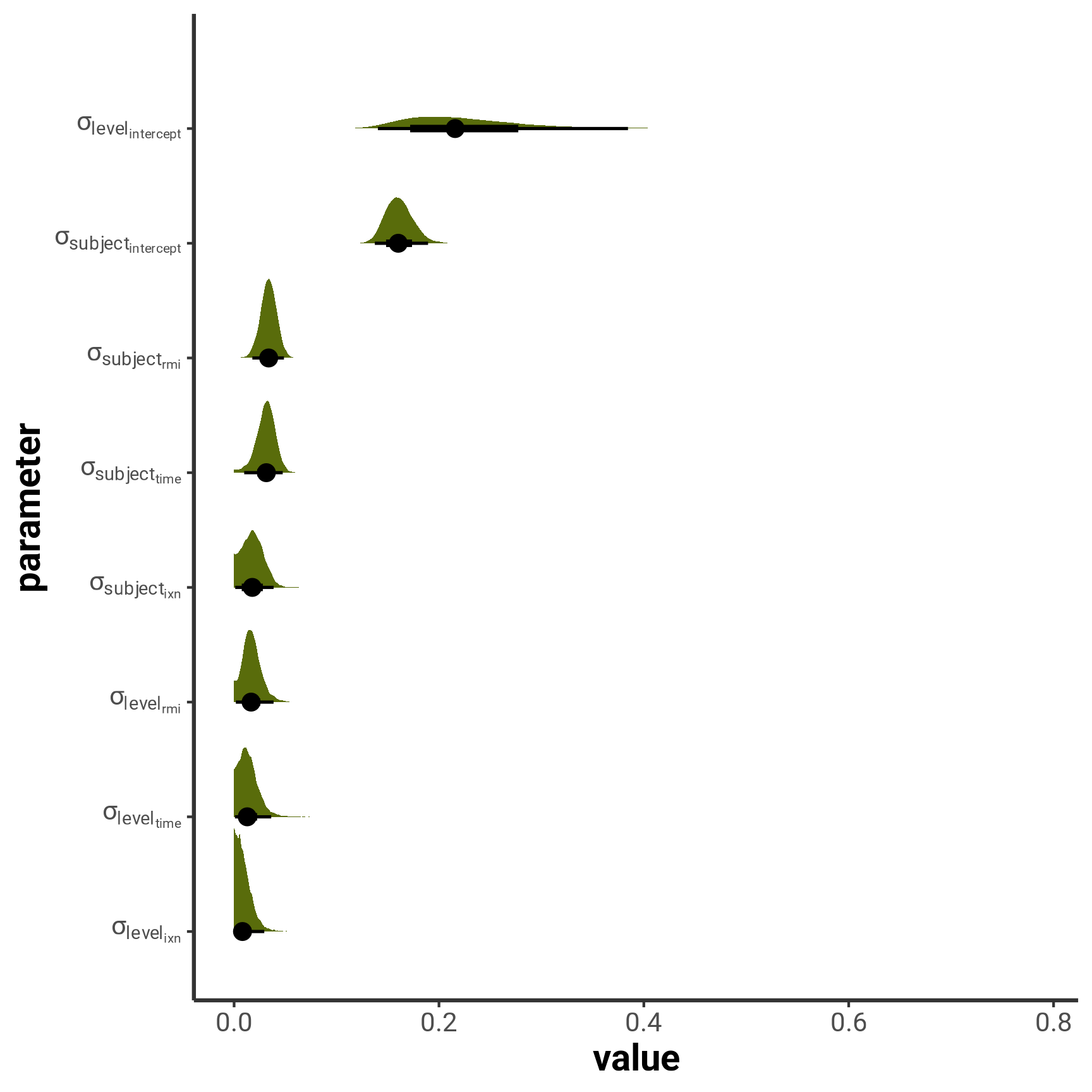
Beta posteriors were shown on the poster, and variance posteriors for each groups’ random effect offsets are shown below.
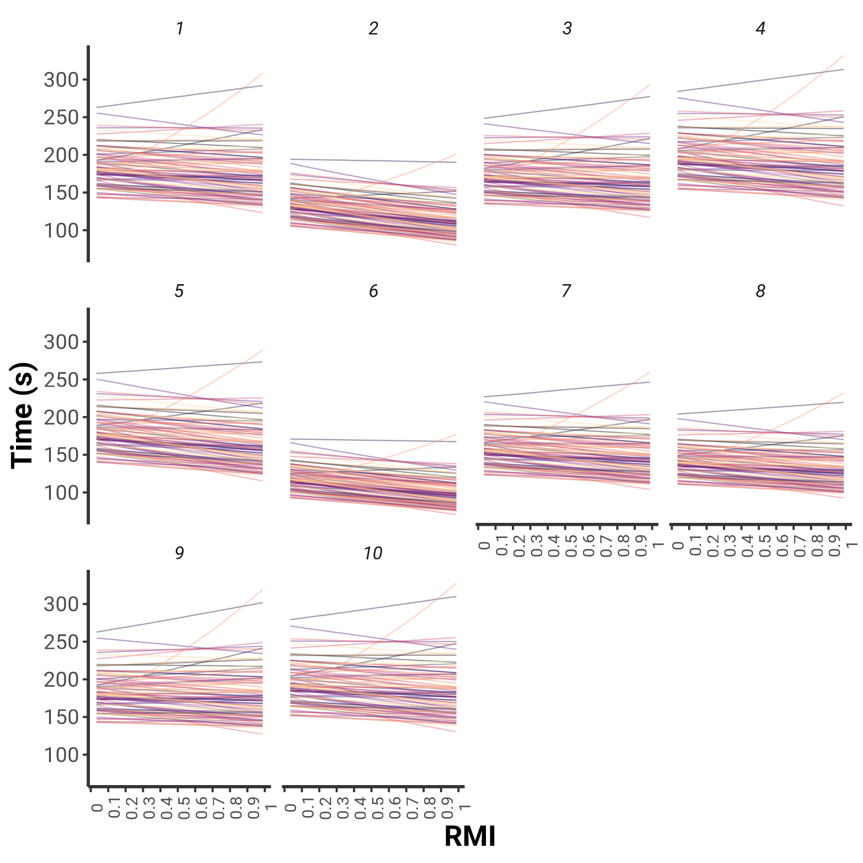
Here is how model predicted relationships varied by subject.
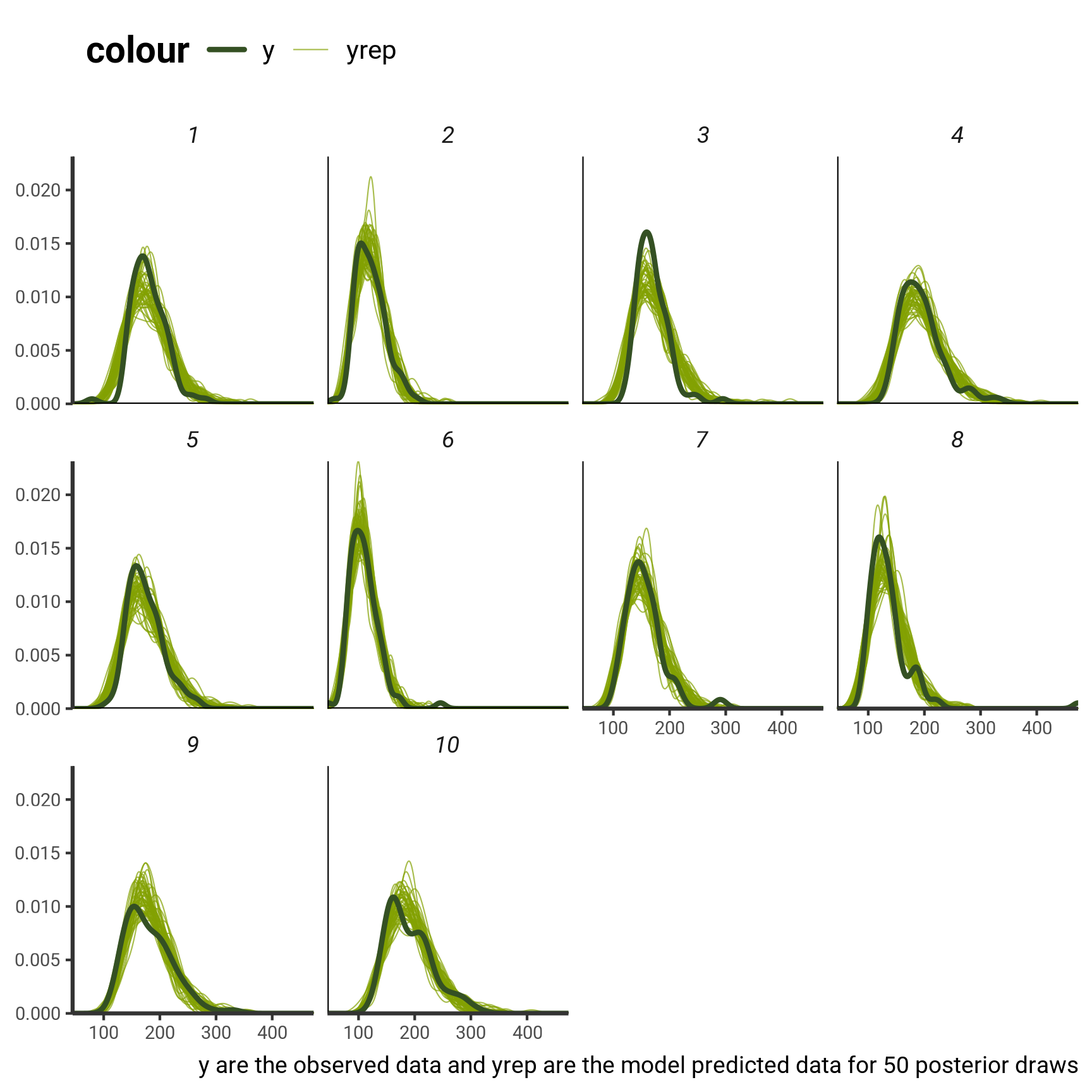
Posterior Predictive Check
Here is a posterior predictive check to validate the model fit to the original data by level.